(Note: if you are familiar with numerical analysis, skip to the "2 Strategies for Initial Guess" section.)
How to Think About the Closest Point on a Spline
One way to think about the problem of finding the closest point on the spline is to imagine that the spline represents a road. We are trying to find the place along the road where the distance from the road to another object on the landscape (let’s say a windmill) is as small as possible. The road may twist back and forth many times. It could approach close to the windmill at numerous points along its length. How do we find which point is the closest? One solution to this problem is to take tiny steps along the road and take a measurement from the road to the object at each step. After walking across the entire road, you can then determine which step was the closest.
Reasons for Finding the Closest Point
Finding the closest point on a spline to another point in the world can be useful for many reasons. Once this point is found, it is easy to determine whether a point or sphere is colliding with any part of the spline path. In Seabird I find the closest point on the spline to one of the birds to determine whether that bird has entered a wind path.
Equation we are Trying to Minimize
Let’s be a little bit more formal with defining our problem. As discussed in the last post, we define the spline using a cubic polynomial with coefficients A B C D. We will use the squared distance between the spline and a point P in the world.

We want to find a parameter x, such that that L as small as possible. This parameter needs to be the smallest that we can find on any segment of the spline.
Minima and Maxima
The type of problem we have is called an optimization problem. If you think of a mathematical function like a landscape, it may have many dips and valleys, as well as hills and mountains. The lowest point in the lowest valley is called a global minimum. A hole in the road might not be the lowest point in a city, but water will still fill the hole when it rains. This is called a local minima (as in the plural form of minimum). This is an important concept, because as we will discuss, it is easy for algorithms to accidentally mistake a local minima for a global minimum.
Short Intro to Newton’s Method
The most common approach to solving minimization problems is a technique called the Newton-Ralphson method, or Newton’s method for short. The idea behind this method is to start with some initial guess for the parameter of the equation, and iteratively refine the guess until we arrive at some value that is hopefully closer to the value we want. The value we are trying to find in Newton’s method is the root of the equation. This is the point where the equation has a value of 0. For instance, in the above equation L would be zero if D were equal to P and the parameter x were 0. An equation may have many roots, or none at all! Because of this, careful use of Newton’s method is necessary to achieve desired results.
Using the Derivative of our Equation
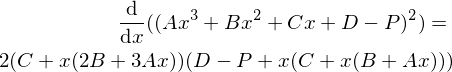
We would like to use Newton’s method to find the minimum of the squared distance equation listed above. However, the squared distance equation we have will not work because it will have no root if the point does not happen to lie directly on the spline. If we are not on the spline, the minimum distance is always greater than zero. And yet, all is not lost! If we take the derivative of the squared distance equation, we can use the fact that there is a root for the derivative at every point where the squared distance equation has a minima and maxima.
Why Newton’s Method is Lousy here
Using the derivative here with Newton’s method becomes troublesome. The derivative indeed has roots, but it has too many roots! This is the problem discussed earlier. Where there are many local minima Newton’s method is likely to get stuck, preventing it from ever finding the global minimum for the function. Not only that, but it will even get stuck at the maxima, because those points on the derivative also happen to be a root.
2 Strategies for Initial Guess
There are 2 main strategies I use for avoiding the problem with Newton’s method getting stuck in local minima and maxima for splines. In the first approach we simply do a linear search over the whole spline, and find which sampled point has the smallest value, and then we run Newton’s method at that point for finer precision.
The second approach is to use the spline parameter we have found from the previous frame for the initial guess on the current frame. For instance, once the bird is moving along the wind path, it is highly likely that the previous parameter is a very good starting guess for the next frame. However you happen to get the initial guess, it is important that the guess is reasonably close to the global minimum.
Using Newton’s Method
Just before we dive into the code, I want to get a little bit more in depth with newton’s method. There is plenty of literature already available for an introduction to how it works. The method is defined like this:
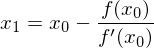
The function f is the function for which we are trying to find a root. We also need f prime, the derivative of the equation to use as the denominator.
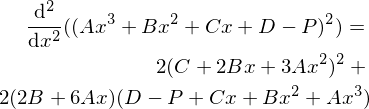
Since we are trying to find the root of the derivative of the squared distance equation, we need to also find the second derivative of the square distance equation so we can use it in Newton’s method as the denominator in the equation.
Here is some example code showing the technique for finding the global minimum by first doing an initial linear search over the spline. First we need the spline segment squared:
1 2 3 4 5 6 | float SplineSegmentSquared(vector A, vector B, vector C, vector D, float x)
{
// (Ax^3 + Bx^2 + Cx + D - P)^2
float segment = A*Power3(x) + B*Power2(x) + C*x + D;
return segment*segment;
}
|
We can then do a consecutive search over the spline to find a rough approximation to the global minimum:
1 2 3 4 5 6 7 8 9 10 11 12 13 14 15 16 17 18 19 20 21 22 23 24 25 | float approximateClosestParam = 0.0f;
float minDistance = FLT_MAX;
const float searchGranuarlity = 0.2f;
for(float i = 0;
i < (float)controlPointCount;
i += searchGranuarlity)
{
int segmentIndex = (int)i; // integer part
float param = i - (float)segmentIndex; // decimal part
float distance = SplineSegmentSquared(coefficients[segmentIndex][3],
coefficients[segmentIndex][2],
coefficients[segmentIndex][1],
coefficients[segmentIndex][0]-point,
param);
if(distance < minDistance)
{
minDistance = distance;
approximateClosestParam = i;
}
}
|
approximateClosestParam will be the rough estimate for the parameter along the spline where it is closest to the point. We can then approximate the parameter using Newton’s method. First we need to implement two more equations, the derivative and second derivative of the spline segment squared:
1 2 3 4 5 6 7 8 9 10 11 | float SplineSegmentSquaredDx(vector A, vector B, vector C, vector D, float x)
{
// Derivative of ((Ax^3 + Bx^2 + Cx + D)^2)
return 2 * (C + x*(2*B + 3*A*x)) * (D + x*(C + x*(B + A*x)));
}
float SplineSegmentSquaredDx2(vector A, vector B, vector C, vector D, float x)
{
// Second derivative of ((Ax^3 + Bx^2 + Cx + D)^2)
return 2 * Power2(C + 2*B*x + 3*A*Power2(x)) + 2*(2*B + 6*A*x) * (D + x*(C + x*(B + A*x)));
}
|
(Note: that I am using a power of 2 on a vector here. This is assumed to be component wise (V.x*V.x, V.y*V.y, etc...)
Then we can run Newton’s method using approximateClosestParam as the initial guess:
1 2 3 4 5 6 7 8 9 10 11 12 13 14 15 16 17 18 19 20 21 22 23 24 25 26 27 28 29 30 31 | const float acceptableError = 1.0e-4f;
const int maxIterations = 3;
float guess = approximateClosestParam;
for(int iteration = 0;
iteration < maxIterations;
iteration++)
{
int segmentIndex = (int)guess; // integer part
float param = guess - (float)segmentIndex; // decimal part
float numerator = SplineSegmentSquaredDx(coefficients[segmentIndex][3],
coefficients[segmentIndex][2],
coefficients[segmentIndex][1],
coefficients[segmentIndex][0]-point,
param);
float denominator = SplineSegmentSquaredDx2(coefficients[segmentIndex][3],
coefficients[segmentIndex][2],
coefficients[segmentIndex][1],
coefficients[segmentIndex][0]-point,
param);
if(fabs(numerator) < 1.0e-4) break; // found root
if(fabs(denominator) < 1.0e-6f) break;
float newGuess = guess - (numerator / denominator);
guess = newGuess;
}
|
Conclusion
Newton’s method is a simple iterative approach; however, it has weaknesses which are particularly evident when working with splines. We can get around these weaknesses with a sufficiently good initial guess; however, it is difficult to determine how good the guess needs to be in a specific case. If you have found a better approach to this problem that works for you, please let me know.
I intended this to be a 3 part series, but it looks like the series will end up being 4 posts. In part 3 I plan to show how to get the total length of the spline. In part 4 I will go over an approach to reparameterizing the spline. After we have done the reparameterization, we can move smoothly along the spline at a continuous speed. This is very useful if we want to control the speed of an animation or motion with spline independently of the shape of the spline. The approach I will discuss has zero real time cost, which makes it appropriate for this blog series.
Resources
Wolfram Alpha has an online derivative solver.
https://www.wolframalpha.com/inpu...of+Ax%5E3+%2B+Bx%5E2+%2B+Cx+%2B+D
A paper to look at for further work on the problems we discussed is Wang, H., Kearney, J., and Atkinson, K., Robust and Efficient Computation of the Closest Point on a Spline Curve.
The approach discussed in this paper combines Newton’s method with quadratic minimization to achieve a better result.
http://homepage.divms.uiowa.edu/~.../CurvesAndSufacesClosestPoint.pdf